For my first visualization, I utilized Palladio and the transatlantic slave voyage database to map the paths of the 3 most active ship captains. Achieving this result required quite a bit of plumbing, as I had to do a great bit of manipulation to make the same rows and columns appear as 3 separate layers on the map. Another challenge was the many duplicate names that I discovered. When I initially sorted by captain name, I found that one of the most common names is William Williams, with 25 trips. However, upon closer inspection, this individual made trips starting in 1725 and ending in 1808. Given the life expectancy of people in that time, especially those at sea, this seemed suspect. I looked closely at the dates and determined that there were effectively three ~10-year ranges for William Williams, suggesting that there were actually 3 captains sharing that name. To fix this I went through the list and broke up all of the names that seemed to have duplicates, and then picked the top 3 names after duplicates were separated.
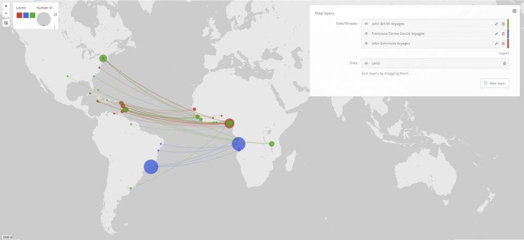
The three different colors represent the 3 captains that are mapped and the size of the dots represents the number of times that they landed at the port. The trips are mapped with the starting location being the place of slave purchase and the ending location being the place of slave landing. This visualization did not provide much insight into the data, as I did not see any trends that warranted further investigation. So after this, I moved on. I included it because I thought it was intriguing.
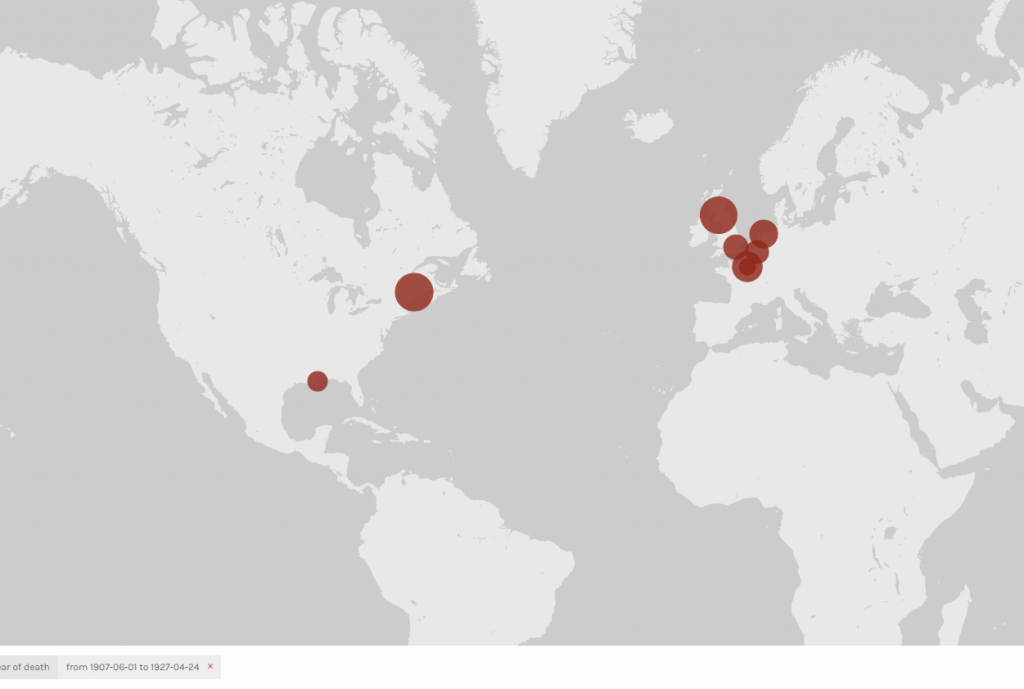
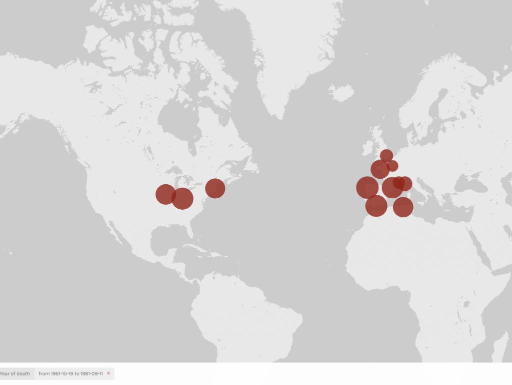
For the second visualization, I mapped the average lifespan of people based on their location, utilizing the sample database inside of Palladio. The dots are sized based on the average lifespan and centered on the respective location. The timeline at the bottom was used to isolate different time periods for comparison. This visualization also required quite a bit of data plumbing, as Palladio only allows the sizing of dots based on the sum of a count, not the average. To get around this, I had to use excel to calculate the partial average so that when Palladio summed it up, the average was accurate. Once the visualization was set up, I noticed a few patterns. I took two different images from different 20-year periods. Between those two periods was a noticeable difference in the size of the dots, indicating that as the years progressed the average lifespan increased. I looked into some of the possible reasons why this could have occurred and discovered multiple major accomplishments in the medical world that could have affected the lifespan of people. Many of these advancements were made by American physicians and scientists, which may explain why the dots in the US are slightly large on average than in Europe (with the exception of some of the larger cities in Europe). In order to take a closer look at this, I created a timeline in Timline.js.
The timeline shows some of the medical advancements that could account for the difference in lifespan.
Drucker’s principal argument is that visualizations are all misrepresentations or “reifications” of information, that are passed off as verbatim presentations. The layer of abstraction and methodology of said abstraction performed by the author or artist is not always shown. I believe this is true. Often the viewer or reader is given a visualization that could be interpreted as truth or fact. The design information that would lead the reader to see and consider the bias of the designer is often omitted or hidden, thereby obfuscating important information. For example with the first visualization that I created, there was a tie for 3rd most active captain. I chose at “random” between the two. Additionally, the latlong data that was used for all of the locations came from a plugin for google drive. Some of the information is inaccurate. At the bottom of the diagram I chose to indicate that I had done this, but I easily could have. If that were the case, a viewer would not know that I manually went into the data and changed locations labeled London from a location in the US to London England. While this is most likely correct, a viewer does not know that I went in and changed that. While I don’t believe I introduced any bias by doing this, I have a western knowledge of geography, which could affect how I fixed the data.
