When I was in the sixth grade, my science teacher had our entire class watch the documentary Super Size Me, a film that follows Director Morgan Spurlock’s month-long social experiment in which he mimicked the lifestyle of a habitual fast-food eater. He did this by (1) eating solely McDonald’s for an entire month and (2) disengaging in all additional exercise (to mirror the average number of steps per day for Americans at 5,000/day). Spurlock also ensured that he tracked how this lifestyle impacts his health by routinely visiting doctors to do weigh-ins and bloodwork and, as one could imagine, Spurlock’s health quickly deteriorated, and the measures were worse than what doctors had predicted. Not only did he gain 24.5 lbs in one month, but he also began experiencing heart palpitations by Day 21. As a sixth grader, I was absolutely appalled, and I vowed never to eat at McDonald’s again (with the exception of the occasional French fries or McFlurries).
Spurlock’s film aimed to shed some light on the fast food industry and its influence over the American public. In watching his film, one might make a quick assumption (as I had) that the consumption of fast food is linked to obesity. As I have gotten older, though, and gained more exposure through courses like sociology about other factors that impact one’s adult life, I have grown a bit more skeptical about the true predictors of obesity. I have learned a lot in college, including within this past semester, not only in my Data Visualization for the Digital Humanities course but also in my other courses as well as in my own life.
In my own life, I am grateful to have things like the ability to attend Bucknell, to fly home for long breaks, and to go out to dinner with friends. At the same time, I’m very aware that not everybody has these same abilities. In fact, not everybody has the opportunity to go to college, and not because they don’t have the grades or because they aren’t smart enough, but because perhaps their mother needs them at home to help with their younger siblings, or to be an additional source of income that will help to pay rent. A lot of what I have discovered during my time at Bucknell is that people – for the most part – are a product of their environment, and thus have different values and skills based off of both how and where they were raised. This explains why when you look at people on Bucknell’s campus, you probably see people who look and behave very differently than those you might observe in the Walmart off of Route 15; it’s no secret that Bucknell’s students are very fitness-oriented.
For my final project, I wanted to take a closer look at this difference in fitness levels. To do this, I worked with the USDA’s Food Environment Atlas dataset, which is a compilation of statistics on food environment indicators with the purpose of stimulating research on the determinants of food choices and diet quality. The USDA collected this data by compiling multiple data sources, such as the 2009 Youth Risk Behavior Surveillance System and the U.S. Census Bureau. The Atlas has three categories of food environment factors: (1) food choices, (2) health and well-being, and (3) community characteristics. Within these categories, there are distinct elements that are considered for each county within the US: access, health, insecurity, restaurants, socioeconomic factors, and access to stores. I chose to explore at least one variable from each of these elements and observe how each of the variables I chose is related to a county’s average obesity rate.
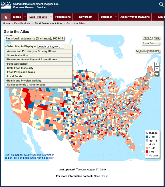
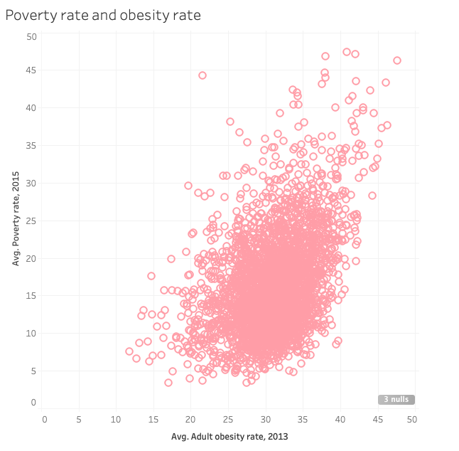
The variables I chose to analyze in relation to a county’s average obesity rate were: the county’s percentage of the population with low access to stores, the county’s median household income, the county’s number of recreation and fitness facilities/1,000 people, the county’s poverty rate, and the county’s percentage of households with food insecurity. Initially, I had included an additional variable that would analyze the obesity rate in conjunction with the number of fast food restaurants/1,000 people, but statistical modeling on this relationship (which I had performed in my statistics class) demonstrated that it is rather insignificant. In fact, modeling this relationship in my statistics class was what inspired me to select this dataset for my final project in Data Visualization, because it made me wonder what the biggest socio-economic predictors of obesity truly are.
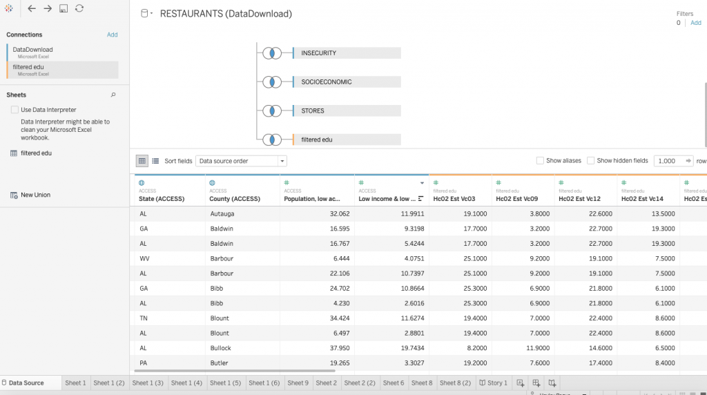
In order to best capture the relationships each of my selected variables has to a county’s obesity rate, I chose to use Tableau for my visualization tool so that I could make use of its mapping and scatter plot functions. I found these to be quite useful and in plotting their relationships I discovered that the only variables that really displayed a significant relationship with county obesity rate were median household income, poverty rate, and average household food insecurity. I was additionally interested in how education played a role in obesity rate but didn’t have the data necessary to explore the relationship, so I met with Carrie to get some assistance. She helped me with obtaining the data, and I did the data plumbing on my own and had a lot of difficulty meshing the two data sources on Tableau. Eventually, I mapped education on its own in just two locations: San Diego (my hometown) and Union County (Lewisburg’s county). This was the result of another suggestion made by Carrie, which was to look at a few locations to compare and contrast them; I chose San Diego and Union County. Taking a closer look at two locations provides the opportunity for “constrained interaction at various checkpoints within a narrative, allowing the user to explore the data without veering too far from the intended narrative” (Segal and Heer, 1147)
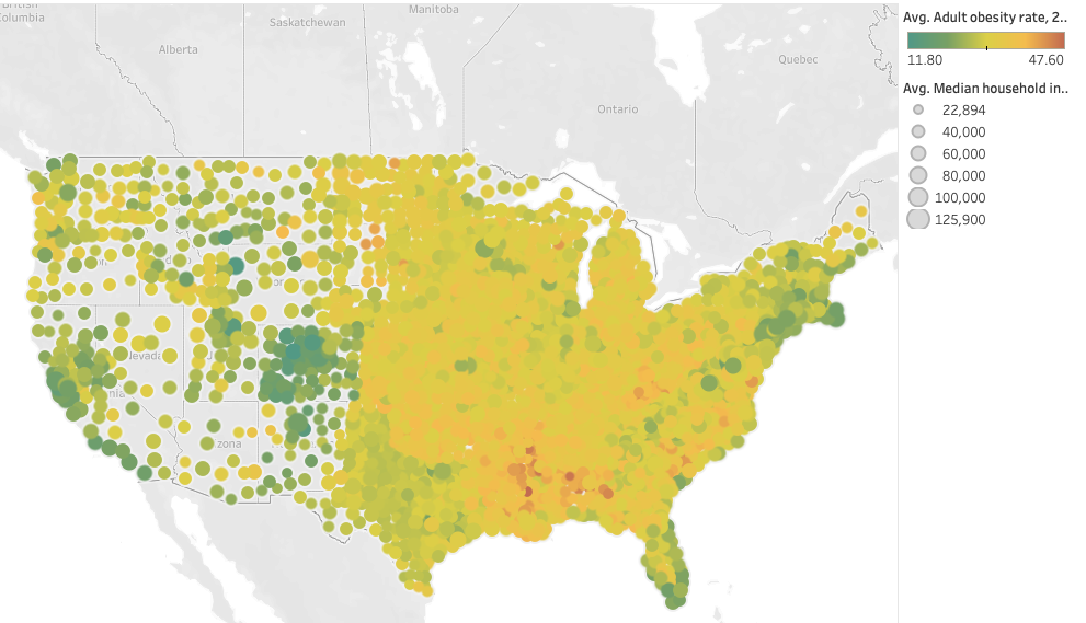
Median household income & obesity rate 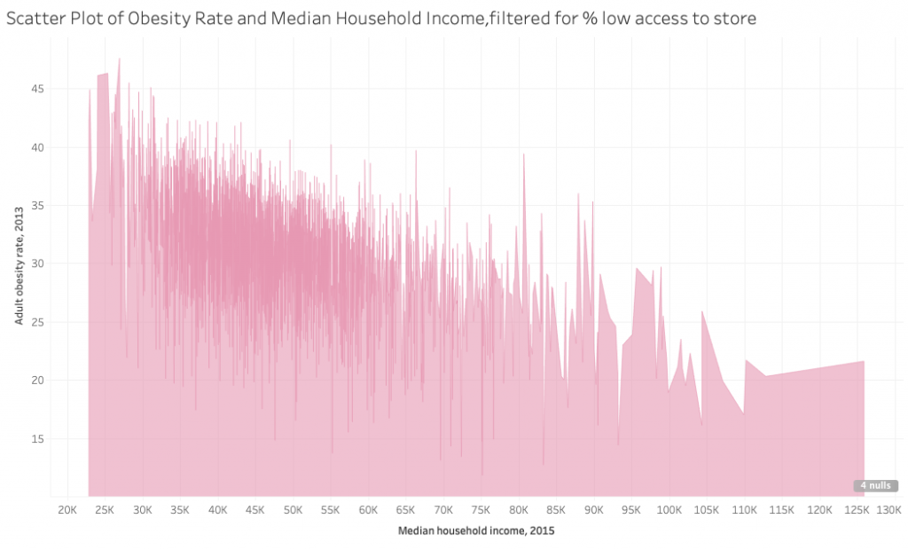
Median household income & obesity rate
Because I am only considering the education levels of people in San Diego and Union County, I cannot make a definitive statement about whether or not education level plays a role in obesity rate. San Diego’s average obesity rate is 19.1% while Union County’s is 28.2%, and I was surprised to find that although San Diego’s percentage of people with a bachelor’s degree or higher was larger than Union County’s at 35.7% versus 20.5%, San Diego also had 7.2% of people aged 25 or above with a 9th grade education or lower compared to Union County’s 5.6% (U.S. Census Bureau). This might indicate that while lower obesity rates are correlated to higher levels of education (which is actually a public statement made by the CDC), higher obesity rates might not be a result of lower levels of education (CDC Morbidity and Mortality Weekly Report).
Although this project could be frustrating at times due to the large amounts of data I was working with, the undependable program I used (lots of crashes!), and my inexperience with data plumbing, I found that I was very comfortable with building a story in data visualization when it was about a topic I am passionate about. I enjoyed using the Food Environment Atlas in both my statistics course as well as this one, because it provided me with a lot of different angles to gather insights from. I believe that looking at visualizations like the one I have created in this project are highly applicable for the real world, particularly for government legislation in determining how best to approach the issue of rising obesity rates. From my data, I would argue that the largest contributor to rising obesity rates isn’t a result of a lack of fitness facilities or from an abundance of fast food restaurants; rather, it’s a result of a lack of social equality and lack of access for those who need it most.
Works Cited
Economic Research Service (ERS), U.S. Department of Agriculture (USDA). Food Environment Atlas. https://www.ers.usda.gov/data-products/food-environment-atlas/
Ogden CL, Fakhouri TH, Carroll MD, et al. Prevalence of Obesity Among Adults, by Household Income and Education — United States, 2011–2014. MMWR Morb Mortal Wkly Rep 2017;66:1369–1373. DOI: http://dx.doi.org/10.15585/mmwr.mm6650a1
Segel, E, and J Heer. “Narrative Visualization: Telling Stories with Data.” IEEE Transactions on Visualization and Computer Graphics, vol. 16, no. 6, 2010, pp. 1139–1148., doi:10.1109/tvcg.2010.179.
U.S. Census Bureau, 2011-2015 American Community Survey 5-Year Estimates