Month: December 2019

This project began with the name Quashie. More specifically it comes from a poem “Quashie’s Verse” I am examining in my master’s thesis. In this poem the poet/ sculptor Quashie negotiates how to create his poem in the shape of a clay jar, as opposed to a traditional verse form like a sonnet, for example. This poem is not only concerned with form but also with measurement. The shape of clay jar embodies the opposition between the linear European system of measure and a more dynamic, indeterminate approach to creating poetry. This idea recalls discussions of timelines and the transition to network theory. Isabel Meirelles succinctly describes the origins and orientation of the timeline: “The first graphical timelines that appeared in the mid-eighteenth century depicted time horizontally, with time moving from left to right … The orientation corresponds to the horizontal preference for depicting time, and the directionality of the authors’ European writing systems. Literature in perception and cognition has shown that we tend to use the direction of our writing systems to order events over time” (Meirelles 88). These are the very systems Quashie attempts to resist with his poetry.

I was happy to engage with network visualization, a form that resists arboreal structures, to understand more about Quashie’s origins. In Palladio I was able to create visualizations of the relations between Quashie and other iterations of the name through time using the African names database. The temporal boundaries were dates of embarkation and disembarkation. What was illuminating was the difference between the visuals depending on the organization of the data. The aesthetics of filtering by disembarkation signified a wholeness or unity among the names with one location and the center of the network. But placing the focus on embarkation created a visual that was truncated and broken, demonstrating the heterogeneity of the ‘origins’ of the names. Recognizing ways that networks could not only show relationships but also map geographies led to my continued exploration of Miller’s poetry in Gephi. 

How does Kei Miller produce invisible maps through his poetry? This question is motivated by Manuel Lima’s statement that “network visualization is also the cartography of the indiscernible, depicting intangible structures that are invisible and undetected by the human eye” (Lima 80). In Gephi I explored how words that signify systems of measure are used beyond “Quashie’s Verse,” mapping the relations between words like “measure” and “distance” in his collection, The Cartographer Tries to Map a Way to Zion. My investigation of the cartography of networks, has been largely motivated by the cartographic concerns of Miller’s poetry collection generally and “Quashie’s Verse” specifically. For this reason, I paid attention to the shapes produced by the community of words among the poems. I borrow from Johanna Drucker’s assertion that “graphic expression is always a translation and remediation” (242). For and I am concerned with demonstrating how data may be understood as an art object and ways that the re-spatialization of the text carries meaning differently from its original form. I was fascinated by the shape produced by the Force Atlas layout, for in the top right corner of the visualization emerges a spider. The spider points toward Anancy, who is constantly metamorphosing from man into spider and back, and he appears several poems across the collection. The Anancy figure is significant, for he is a trickster who plays with and plays on language, and on an epistemological level invokes an endless play of signifiers. Then, seeing a version of Anancy appear in this new map prompted me to think more about how maps can be visible or invisible, and ways that lines, measurements and algorithms may be humanistic.

My project, then, picks up where I left off with Gephi. While I am interested in this unfamiliar or distant way of approaching my reading of Miller’s collection, I find it valuable to create a more nuanced picture or map of relations using tools that allow me to engage with the poetry in their original form. First, I turned to Poemage, a visualization tool for exploring the “sonic topology” of a poem. I am interested in visualizing the relationships between sounds in the poems that include Quashie. While Gephi allowed me to draw or create a map of relationships between specific words in the collection, Poemage allows me to create a map between specific sounds in individual poems. Using these tools, I analyze the shapes that emerge from mapping the relationship between words and sounds in the collection and within the poems. To accomplish this, I do a combination of close reading and distant reading to produce what Tanya Clement calls a differential reading. She notes that this method “defamiliarize[s] texts, making them unrecognizable in a way (putting them at a distance) that helps scholars identify features they might not otherwise have seen, make hypotheses, generate research questions, and figure out prevalent patterns and how to read them” (2). In addition to Poemage I use Voyant to get a view that combines the closeness with the text that Poemage fosters and the distance from the text that Gephi offers, allowing me to engage with The Cartographer Tries to Map a Way to Zion in both familiar and unfamiliar ways.

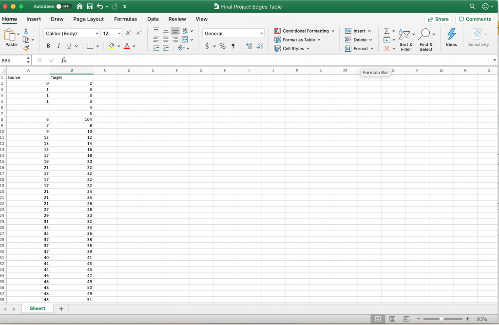
I also wanted to continue exploring network visualization and analysis in Miller’s collection with Gephi. With that I turn to the field of geocriticism, where “To draw a map is to tell a story in many ways and vice versa” (Tally 4). The narrative between the cartographer and the rastaman not only tells a story, it also draws a map. Since the writing of the poems function to create maps I decided to extend the community of words I map to words related to poetry and verse. To do this I appended my initial nodes and edges table to include words like “shape”, “draw”, and “lines,” along with the poems they appear in. To create a more fulsome picture of the mapping relationships, I also decided to include all the iterations of the word “map” in my dataset.

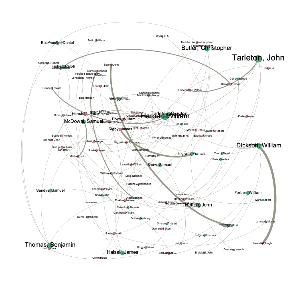
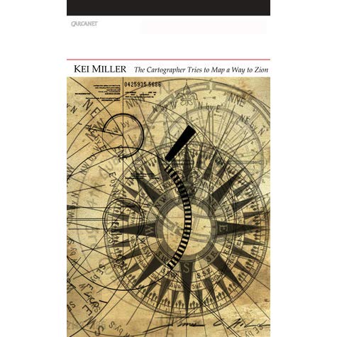
In Gephi the image produced using Force Atlas has a striking resemblance to a compass. I noticed this because there is a compass on the cover of The Cartographer Tries to Map a Way to Zion. 

• 

• 

An important distinction between the two is that in my design the rastaman at the center. This displaces the cartographer as the symbolic figure of mapping and map design. The visualization I created also demonstrates the play between each of the character’s operations. Insightfully, in “xx” the cartographer states that “every language, even yours, / is a partial map of this world” (2-3). Comparing the first network to the second one I produced in Gephi, it becomes clear that the first – with fewer nodes and edges – is indeed a partial map of the collection. But the same could be said of the second one, as the biases of my own research (specific words) implicate the resulting image. No one view or perspective is definitive. This motivated me to see what may be revealed if I changed the layout.

• 

• 

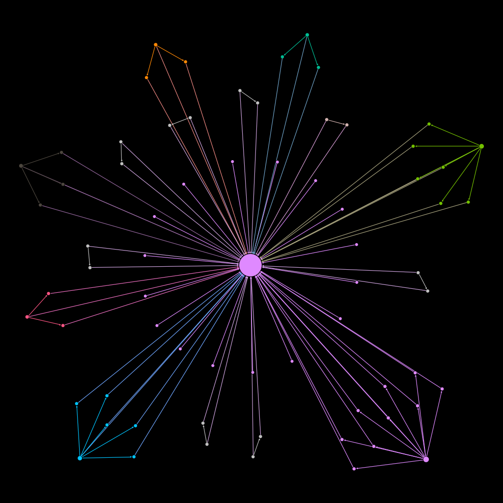
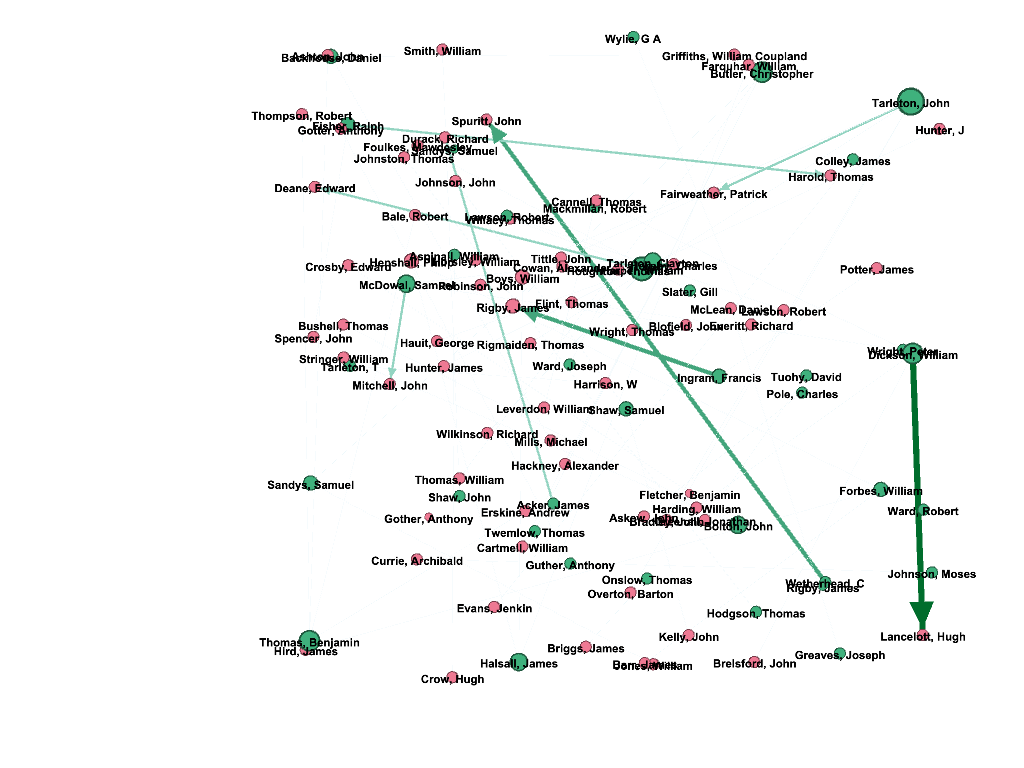
I created the second visualization using the Fruchterman Reingold layout to demonstrate the diverse relationship between the different words in The Cartographer Tries to Map a Way to Zion. Each word is customized to have a distinct color. I used the custom palette to color the nodes with browns and neutral tones in an attempt to mimic the cover image. But I ultimately decided to switch the palette to a variety of bright colors in order to illustrate the variety of words that make up this map as opposed to uniform colors that risk implying there is uniformity in navigating through a space or place. 

I understand the following visualization to operate as a compass, not necessarily to orient the viewer within the collection but to point toward its complexities in a nonlinear way. 

Though seeing the relationship between the variety of words in a network diagram is illuminating, I had the desire to map some of these words in their individual contexts. When I first tried using Poemage I was interested to use the tool to investigate “Quashie’s Verse” especially because of the distinct shape it has. However, after fiddling with the poem in a plain text file I discovered that the formatting in the program did not substantially change.

• 

• 

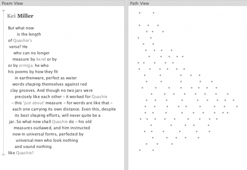
Instead I focused on a poem that also included Quashie, crafting poetry and rhythm. Miller’s “xvii” replicates a dub poem, which is a form of performance poetry that incorporates a beat, usually from a drum – this made it a good candidate for Poemage. After uploading the poem to the program, I decided to focus on assonance. Doing this sort of distant reading allowed me to see a sonic pattern; I noticed the lines that connected words with an “ae” sound.

This prompted me to think more about the relationship between “rastaman”, “iambic” and “Quashie.” When considering Quashie’s project of writing with a verse form intuitive to him instead of the way he has been “instructed / now in universal forms” generates similarities between his task and that of the rastaman (17-18). Both of these men resist what the iambic metre represents. Playing on the meaning of metre as a unit of measure to create maps and a measure with which one crafts poetry is not only a way to showcase the rigidity traditionally associated with these endeavors, it also links these elements in a way that resists it. The use of assonance is then a way that Miller creates an invisible map, for he also takes space into consideration (even outside of his concrete poem). With Poemage I noticed the even line spacing between those instances of “rastaman”, “iambic” and “Quashie.” Each of the words frame the repeated “DUP-dudududu-DUP-DUP” sound, which speaks to the departure from the iambic metre with one that is intuitive to the speaker/rastaman. Moreover, this highlights the relationship between the rastaman and Anansi in illustrating a “partial map” of Jamaica, one that is not seen by the cartographer, and figures that represent this mathematical, objective and even colonial perspective. 

This examination was so fruitful in augmenting the work I began with Gephi that I was excited to use Voyant. The corpus consists of each of the thirteen poems that contain a version of the word “map.” After transcribing a few of the poems to experiment with in poemage I continued to put each of the poems in their own plain text files to upload them to Voyant Tools. I had the idea to visualize the “map” in Voyant spatially. This idea came from my experience negotiating whether to distinguish “map” from “mapped” and “mapping” in the nodes table for Gephi and their frequencies within a single poem. Using a text analysis tool lends itself to working with the text in its ‘whole’ form and observing trends within the entire corpus. In this way Voyant kind of combines my desire to think about the collection as well as the individual poems by examining how a group of these poems relate to each other.

The Trends graph allowed me to see the most frequent words in the corpus, two of which included “map” and “maps.”  I also used the cirrus tool to visualize the relative frequencies of words in the shortest poem. Despite its short length, it contains one of the most significant lines in the collection and to my argument: “I will draw a map of what you never see” (19). It is ironic that some of the smallest words are “bigger” and “larger” while one of the bigger ones is “guess.” I believe this speaks to the pivotal place of indeterminacy in the way the rastaman (and Quashie) understands mapping. It also calls an important connection into sharper focus; the shortest poem is the one that contains the largest number of the word “map.”

Thinking about this interesting occurrence, prompted me to consider using a tool within Voyant to visually contextualize the appearance of “map” and “maps.”

Like the Gephi Force Atlas layout, if one looks closely this Word Tree visualization also resembles a spider. The repetition of the spider speaks to the network that a spider like Anancy would produce by spinning his web. This web is a complex one, made up of words, and like many spider webs remain nearly invisible to the human eye. Flexing my design skills in Gephi and making use of the built-in algorithms in Poemage and Voyant I am able to show several versions of the (in)visible maps that Kei Miller creates through his poetry.

Works Cited

Clement, Tanya. and Price, Kenneth M. “Text Analysis, Data Mining, and Visualizations in Literary Scholarship.” Text Analysis, Data Mining, and Visualizations in Literary Scholarship, 2013.

Drucker, Johanna. “Graphical Approaches to the Digital Humanities.” Schreibman, Susan, et al. A New Companion to Digital Humanities. Chichester, West Sussex, UK, 2016.

Lima, Manuel. Visual Complexity: Mapping Patterns of Information. Princeton Architectural Press, 2011.

Meirelles, Isabel. Design for Information : An Introduction to the Histories, Theories, and Best Practices Behind Effective Information Visualizations. Rockport, 2013.

Miller, Kei. The Cartographer Tries to Map a Way to Zion. Carcanet, 2014. 

Tally, Robert T. Topophrenia: Place, Narrative and the Spatial Imagination. Indiana UP, 2019.  

Link to Visualization https://public.tableau.com/profile/aung.pyae.phyo#!/vizhome/APPDataVizFInal/3?publish=yes

Website Link

Ever since my first year at Bucknell, I’ve been really interested in the patterns of international students pursuing higher education in the United States. I wanted to know why people would travel all the way to the middle of Pennsylvania for their future. I knew why I came to Bucknell, a decision that was made with the consultation of my high school, research into my field of study and the uniqueness of the program I wanted to go for. Interested in this, I take a look into the information available online, I only found the factbook, which had information, but it was not interactive in any way, and was very hard to get through because it was all numbers. The information was also focused a long term institutional outlook rather than a student-focused study. During in-class consultations, Agnes had suggested looking at the University’s interactive dashboards for data. Looking at these sources, they were not as specific about the international community at Bucknell as I wanted to see.

So for my final project, I wanted to take a look at five years’ worth of international student data, from the class of 2019 to 2023. My initial idea when I started thinking about this project was to make a Bucknell international student-specific infographic showing where we were from and how the community has grown over this five-year period. The data that I used for the project was obtained from the International Student Services at Bucknell. The information contains the student’s gender, class year, college within Bucknell, major, country of origin, their high school, and the category of their field of study. Within the data, I have the information of 279 students total. Data plumbing was minimal, as all I had to do was combine append the data of all international students in the academic year 2019-2020 with the data of seniors from the academic year before.

To interpret the data, I wanted to use Tableau to look at the demographics, and make the results interactive, with the user able to change various settings to look at their own specific research questions. Furthermore, I also wanted to look into the connections between high school and enrollment, to see how much secondary education mattered when choosing a college. To do this, I chose to use Gephi and map out connections between the students. The final tool I wanted to use was Timeline JS, to build a timeline about the international students at Bucknell in context to global events. By employing all three tools, I hope to effectively show a more complete look on the international student population with more interesting insights.

For the tableau visualizations, I was thinking about what people might be interested in when they think about international students. In a lot of demographics infographics, we are represented as a number of countries or a percentage statistic. It’s not wrong to do so, it comes up as fascinating data. I just wanted to make sure that my infographic would convey the same information, but in a way that I feel makes me feel personally visible. This is where Tableau’s symbol map comes into play. Throughout my survey of infographics, that was the most visually engaging methods of communicating the international demographic. It also is a great way to highlight the countries that are not represented as well.

Tableau is also the final part of my infographic. By ending on an interactive visualization that gives you tools to play around and explore the data, I want to encourage others to become knowledge generators themselves, to have their small research questions easily explorable. By using the martini glass structure, I hope to take the viewers through my narrative to inform them about what the dataset is and inspire them on what can be done with the final visualization, allowing for free exploration on a path of their choice.

My first foray into the project was the Gephi component, which I was most interested in. My decision to look at Bucknell as an option was mainly because I knew students from my high school who went to Bucknell. To that end, I set out to connect people who came from the same high school, and gave them more weight if they belonged to the same year. After building the edge table, I used the Radial Axis Layout, grouping the nodes by class year. This produced a visualization that, in my opinion, created a pretty strong argument that the high school that an international student went to plays a significant part in deciding if future students apply. Of course, this dataset only contains the number of students who are enrolled, and not those that apply, and thus, this factor might have meaning if looked at in a college application context rather than in a college enrollment context.

For the final part of the project, I wanted to put in a timeline that shows some important events that influenced higher education in the US, Bucknell University, and international students who want to pursue a degree in the US. These events required more research (and from time of writing, more events that actually impacted international students.) For now, major events have been highlighted, and I hope to continue on this project and add more later on.

Working with this project was an interesting exercise in the release of data. I spent a lot of time thinking about how not to single people out because of how unique individuals can be in a small dataset. Due to the low number of international students at Bucknell, it became a scramble to try to find ways to hide the information that was unique enough to identify the individual student. Around half of international students are the only one from their own country, and while their country being represented is not a problem, the other data that comes with the dataset would not be appropriate to release.

Through this project, I think that I have been able to dive into the datasets that I received to produce some interesting visualizations. In particular, Gephi has really helped in my search for an answer about the correlations between enrollment and high school. Tableau has also opened up the path to be interactive with the data and let the readers decide what they want to explore. By being able to employ these tools, I believe that I have created an interface that will help people make their own visualizations, and creating more knowledge generators.

When I was in the sixth grade, my science teacher had our entire class watch the documentary Super Size Me, a film that follows Director Morgan Spurlock’s month-long social experiment in which he mimicked the lifestyle of a habitual fast-food eater. He did this by (1) eating solely McDonald’s for an entire month and (2) disengaging in all additional exercise (to mirror the average number of steps per day for Americans at 5,000/day). Spurlock also ensured that he tracked how this lifestyle impacts his health by routinely visiting doctors to do weigh-ins and bloodwork and, as one could imagine, Spurlock’s health quickly deteriorated, and the measures were worse than what doctors had predicted. Not only did he gain 24.5 lbs in one month, but he also began experiencing heart palpitations by Day 21. As a sixth grader, I was absolutely appalled, and I vowed never to eat at McDonald’s again (with the exception of the occasional French fries or McFlurries).

            Spurlock’s film aimed to shed some light on the fast food industry and its influence over the American public. In watching his film, one might make a quick assumption (as I had) that the consumption of fast food is linked to obesity. As I have gotten older, though, and gained more exposure through courses like sociology about other factors that impact one’s adult life, I have grown a bit more skeptical about the true predictors of obesity. I have learned a lot in college, including within this past semester, not only in my Data Visualization for the Digital Humanities course but also in my other courses as well as in my own life.

In my own life, I am grateful to have things like the ability to attend Bucknell, to fly home for long breaks, and to go out to dinner with friends. At the same time, I’m very aware that not everybody has these same abilities. In fact, not everybody has the opportunity to go to college, and not because they don’t have the grades or because they aren’t smart enough, but because perhaps their mother needs them at home to help with their younger siblings, or to be an additional source of income that will help to pay rent. A lot of what I have discovered during my time at Bucknell is that people – for the most part – are a product of their environment, and thus have different values and skills based off of both how and where they were raised. This explains why when you look at people on Bucknell’s campus, you probably see people who look and behave very differently than those you might observe in the Walmart off of Route 15; it’s no secret that Bucknell’s students are very fitness-oriented.

For my final project, I wanted to take a closer look at this difference in fitness levels. To do this, I worked with the USDA’s Food Environment Atlas dataset, which is a compilation of statistics on food environment indicators with the purpose of stimulating research on the determinants of food choices and diet quality. The USDA collected this data by compiling multiple data sources, such as the 2009 Youth Risk Behavior Surveillance System and the U.S. Census Bureau. The Atlas has three categories of food environment factors: (1) food choices, (2) health and well-being, and (3) community characteristics. Within these categories, there are distinct elements that are considered for each county within the US: access, health, insecurity, restaurants, socioeconomic factors, and access to stores. I chose to explore at least one variable from each of these elements and observe how each of the variables I chose is related to a county’s average obesity rate.

The variables I chose to analyze in relation to a county’s average obesity rate were: the county’s percentage of the population with low access to stores, the county’s median household income, the county’s number of recreation and fitness facilities/1,000 people, the county’s poverty rate, and the county’s percentage of households with food insecurity. Initially, I had included an additional variable that would analyze the obesity rate in conjunction with the number of fast food restaurants/1,000 people, but statistical modeling on this relationship (which I had performed in my statistics class) demonstrated that it is rather insignificant. In fact, modeling this relationship in my statistics class was what inspired me to select this dataset for my final project in Data Visualization, because it made me wonder what the biggest socio-economic predictors of obesity truly are.

In order to best capture the relationships each of my selected variables has to a county’s obesity rate, I chose to use Tableau for my visualization tool so that I could make use of its mapping and scatter plot functions. I found these to be quite useful and in plotting their relationships I discovered that the only variables that really displayed a significant relationship with county obesity rate were median household income, poverty rate, and average household food insecurity. I was additionally interested in how education played a role in obesity rate but didn’t have the data necessary to explore the relationship, so I met with Carrie to get some assistance. She helped me with obtaining the data, and I did the data plumbing on my own and had a lot of difficulty meshing the two data sources on Tableau. Eventually, I mapped education on its own in just two locations: San Diego (my hometown) and Union County (Lewisburg’s county). This was the result of another suggestion made by Carrie, which was to look at a few locations to compare and contrast them; I chose San Diego and Union County. Taking a closer look at two locations provides the opportunity for “constrained interaction at various checkpoints within a narrative, allowing the user to explore the data without veering too far from the intended narrative” (Segal and Heer, 1147)

• 

• 

Because I am only considering the education levels of people in San Diego and Union County, I cannot make a definitive statement about whether or not education level plays a role in obesity rate. San Diego’s average obesity rate is 19.1% while Union County’s is 28.2%, and I was surprised to find that although San Diego’s percentage of people with a bachelor’s degree or higher was larger than Union County’s at 35.7% versus 20.5%, San Diego also had 7.2% of people aged 25 or above with a 9^th grade education or lower compared to Union County’s 5.6% (U.S. Census Bureau). This might indicate that while lower obesity rates are correlated to higher levels of education (which is actually a public statement made by the CDC), higher obesity rates might not be a result of lower levels of education (CDC Morbidity and Mortality Weekly Report).

Although this project could be frustrating at times due to the large amounts of data I was working with, the undependable program I used (lots of crashes!), and my inexperience with data plumbing, I found that I was very comfortable with building a story in data visualization when it was about a topic I am passionate about. I enjoyed using the Food Environment Atlas in both my statistics course as well as this one, because it provided me with a lot of different angles to gather insights from. I believe that looking at visualizations like the one I have created in this project are highly applicable for the real world, particularly for government legislation in determining how best to approach the issue of rising obesity rates. From my data, I would argue that the largest contributor to rising obesity rates isn’t a result of a lack of fitness facilities or from an abundance of fast food restaurants; rather, it’s a result of a lack of social equality and lack of access for those who need it most.

Works Cited

Economic Research Service (ERS), U.S. Department of Agriculture (USDA). Food Environment Atlas. https://www.ers.usda.gov/data-products/food-environment-atlas/

Ogden CL, Fakhouri TH, Carroll MD, et al. Prevalence of Obesity Among Adults, by Household Income and Education — United States, 2011–2014. MMWR Morb Mortal Wkly Rep 2017;66:1369–1373. DOI: http://dx.doi.org/10.15585/mmwr.mm6650a1

Segel, E, and J Heer. “Narrative Visualization: Telling Stories with Data.” IEEE Transactions on Visualization and Computer Graphics, vol. 16, no. 6, 2010, pp. 1139–1148., doi:10.1109/tvcg.2010.179.

U.S. Census Bureau, 2011-2015 American Community Survey 5-Year Estimates

I initially became intrigued with the ship, the Mary, after being introduced to the Trans-Atlantic Slave Trade Database in the beginning of the semester. I wanted to know more about the specific ship and what it could tell me when it was separated from the records in the database. This concept was inspired by the argument made by Segel and Heer: “while stories often concern interacting characters, they may also present a sequence of facts and observations linked together by a unifying theme or argument” (Segel & Heer), and ultimately led me to my research question: what happens to the hairball of Trans-Atlantic Slave Data when I drill down and look at a particular ship? In order to answer my question, I had to rely on several digital visualization methodologies that I learned in class this semester because each helped me approach the question from a different angle.

First, I used ArcGIS Online to map the voyages that the Mary took. I created a dataset that consisted of the place of origin for each voyage, the place where the slaves were purchased, and the place the slaves landed. I then had to create a map layer for each set of locations before merging them all together, so that the path taken would show up all on one layer. ArcGIS allowed me to visually illustrate the slave trade and the route that the Mary took. Using the heat map feature, I was able to see that Liverpool,  Bonny, and New York were some of the most common places that the Mary visited.

 I was then able to drop down pins in those locations and draw lines connecting them to really demonstrate the path the Mary often took. I ran into some difficulty when trying to map the ports on the basemap because the geographical category varied for each location in the Trans-Atlantic Slave Database. Some records used states to share where the Mary went, while others used countries or cities. However, I was able to overcome this by putting a pin on the locations of the ports in the present day, which is pretty accurate.

After learning what ports the Mary often went to, I wanted to know more about each location and their significance in the greater Trans-Atlantic Slave Trade. I felt that storymap platform in ArcGIS would best help me convey the story of the Mary because it allowed me to tell the story around each of the locations on the map. I had key locations (Liverpool, Bonny, and New York) on the Trans-Atlantic Slave trade and needed to be able to tell the story of them. Through this process, I learned that not only was Liverpool a common port of origin for the Mary, but it also had a significant role in the Trans-Atlantic Slave Trade. I felt that using ArcGIS was an effective way of addressing my research question, especially because I was working with many locations so the map visual was very beneficial. I found this correlation extremely intriguing and decided to do some more research into the relationship. I learned that the Mary was built in Liverpool too! This finding led me to start researching into the owners of the Mary and the various captains of each of the Mary’s journeys. I thought it would be really interesting to learn about each of these individuals and what their role was in the greater Trans-Atlantic Slave trade. I also wanted to see what their relationships were to each other and how those connections could have impacted events that occurred during that time period. 

However, I immediately ran into problems when I went back to the database on a quest for more information. I found that because ‘Mary’ is a very common name, there could have been numerous ships with the same name and there was no reliable way of differentiating the ships. There were 243 recorded voyages under the vessel name ‘Mary.’ between the years of 1649 and 1816. However, since my focus was on Liverpool, I filtered the data to only show voyages that began out of Liverpool, which totaled 186. In order to discover the relationships between the different individuals, I had to create a new dataset that included the owner(s) name(s) and the captain(s) name(s).

I felt that Gephi would be the best digital visualization methodology to show the relationships among captains and owners of the Mary because the visualizations I can create in Gephi are “the cartography of the indiscernible, depicting intangible structures that are invisible and undetectable to the human eye” (Lima 80). In order to use the platform, I had to again manipulate my data. However, this is where I ran into another problem. For some of the Mary’s voyages, there were multiple owners and multiple captains listed, but Gephi limited me to only using one owner and one captain. To keep things consistent, I used the owner whose name was listed first and the captain whose name was listed first for every voyage. I created a node table, where I listed all of the Mary’s captains and owners. I then inserted the spreadsheet into Gephi and each individual received their own id number. Next, I manually connected the owner of the ship listed for each individual voyage (source) to the captain of the same voyage (target) using each individual’s unique Id number, creating an edge table. Once I uploaded the edge table, I was able to work with the data.

I created a network of people and differentiated the captains from the owners of the ship by making the nodes representing captains pink and owners green. I used the modularity calculation to see if there was a nexus of names that were closely related and then I used the average degree calculation to see how many relationships each individual had. In the visualization I created I made the size of each node represent the degree, so the larger the node, the more relationships a person had. Also, I weighed the edges to represent the strength of the relationship between two individuals using the principal Graham mentioned: “weight is a numeric value quantifying the strength of a connection between two nodes” (Graham 206). Since there is no ‘undo’ button in Gephi, I continued to manipulate my data to see what else I could learn from it. I used numerous different filters and partitioned my results by degree, in-degree, and modularity.

The visualizations I created in Gephi gave me the ability to draw conclusions and see similarities/differences within the data set that I was unable to see in a typical spreadsheet format. Not only did I learn that where a node is in relation to other nodes mattered, but that the weight of the edge between them is also significant. I was able to see certain patterns that I may not have noticed prior that I can further dive into.

I feel that both Gephi and ArcGIS allowed me to narrow down and focus on just the Mary. These platforms gave me the ability to really illustrate the story of the Mary and learn about the numerous people, places, and purposes that went along with it. My findings helped me get a better understanding of the greater Trans-Atlantic Slave trade because I was able to draw connections and see relationships that I would not have previously picked up on.

Link to my WordPress Site: The Mary